TL;DR:
- Supply and demand determine market prices through the intersection of curves that represent quantity buyers want and sellers offer. Price adjustments occur due to surpluses or shortages, influenced by shifts in the curves caused by external factors like income or production costs. Price controls such as ceilings and floors can disrupt this balance, creating shortages or surpluses in the market.
Supply and demand is the basic market rule that price moves until the amount buyers want equals the amount sellers offer. When those two quantities match, the market reaches equilibrium, expressed simply as Qd = Qs (quantity demanded equals quantity supplied). Two laws govern this: the law of demand states that as price rises, buyers want less; the law of supply states that as price rises, sellers offer more. Throughout this guide, you'll see both laws at work in everyday U.S. examples, from gas stations to concert venues, and you'll get a chance to test the ideas in an interactive simulator.
Table of Contents
- How do supply and demand curves work?
- How does equilibrium price form in a real market?
- What causes a curve to shift vs. move along its path?
- Why do price ceilings cause shortages and price floors cause surpluses?
- Why does elasticity change how markets respond?
- Real U.S. examples that bring the theory to life
- Common misconceptions beginners should watch out for
- How do economists actually measure supply and demand?
- Try the interactive supply and demand simulator yourself
- Key Takeaways
- Why supply and demand still matters outside the classroom
- See equilibrium move in real time with Apexapro
- Useful sources for further reading
How do supply and demand curves work?
Every supply-and-demand diagram shares the same skeleton. Price runs up the vertical axis; quantity runs along the horizontal. The demand curve slopes downward from left to right, because buyers are willing to purchase more only when the price falls. The supply curve slopes upward, because higher prices give producers a stronger incentive to bring goods to market.

Where the two curves cross is the market equilibrium, the single price-quantity combination where buyers and sellers are both satisfied. At that intersection, Qd = Qs, and there is no pressure for price to move.
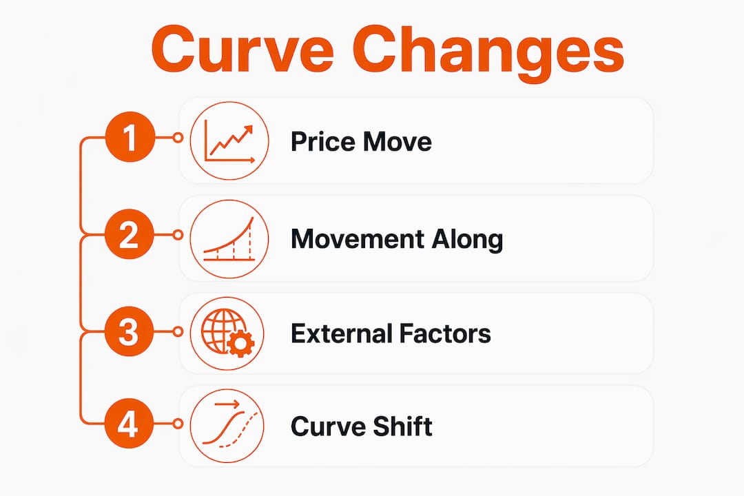
Two types of change look similar on a graph but mean very different things:
- Movement along a curve happens when price changes and quantity responds, with everything else held constant. Trace your finger up or down the existing line.
- A shift of the curve happens when something other than price changes, such as income, tastes, or production costs. The entire line moves left or right.
Pro Tip: Draw the axes first, then sketch the curves freehand. Label the equilibrium point E and mark the equilibrium price P* and quantity Q* before adding any shifts. That habit alone prevents most graphing errors on exams.*
How does equilibrium price form in a real market?
Equilibrium is not a fixed destination. It is a dynamic price-discovery process where surpluses and shortages constantly push prices toward balance.
Consider two quick scenarios. Suppose a retailer prices a new gadget above the equilibrium. Shelves fill up, warehouses overflow, and the retailer eventually cuts the price to move inventory. That excess stock is a surplus. Now flip it: the retailer prices the gadget below equilibrium. Shoppers line up, stock runs out by noon, and the retailer raises the price to ration the remaining units. That empty shelf is a shortage.

According to OpenStax Principles of Economics, at a price above equilibrium there is excess supply; below equilibrium there is excess demand. Prices then adjust toward equilibrium.
What causes a curve to shift vs. move along its path?
A movement along a curve has one cause: a price change. A shift of the curve has a different cause entirely, something that changes buyer or seller behavior at every price level.
Demand shifters
These factors move the entire demand curve left or right:
- Income: When household incomes rise, demand for most goods increases. A recession does the opposite.
- Tastes and preferences: A viral social media trend can spike demand for a product overnight.
- Prices of substitutes and complements: If beef prices jump, demand for chicken rises. If gas prices soar, demand for large SUVs often falls.
- Expectations: Consumers who expect prices to rise next month buy more today.
- Population: More people in a market means more total demand.
Holiday shopping is a textbook demand shifter. Every November, demand for toys and electronics shifts right, pushing prices up before retailers discount in January.
Supply shifters
These factors move the entire supply curve left or right, and they are the core of factors affecting supply:
- Input costs: When lumber prices spike, homebuilders supply fewer houses at any given price.
- Technology: Better harvesting equipment lets farms produce more corn at lower cost, shifting supply right.
- Number of sellers: New competitors entering a market expand total supply.
- Weather and natural events: A drought cuts crop yields; a hurricane disrupts refinery output.
- Taxes and subsidies: A new excise tax raises production costs and shifts supply left; a government subsidy does the opposite.
COVID-era supply disruptions illustrated this sharply. Factory shutdowns and shipping bottlenecks shifted supply curves left across dozens of industries simultaneously, driving prices higher until supply chain dynamics gradually normalized.
Why do price ceilings cause shortages and price floors cause surpluses?
A price ceiling set below equilibrium causes a shortage. A price floor set above equilibrium causes a surplus. Both outcomes follow directly from the surplus-shortage logic above.
Rent control is the classic ceiling example. When a city caps apartment rents below the market rate, more people want to rent than landlords are willing to supply at that price. The result is a persistent housing shortage: long waitlists, under-the-table fees, and reduced incentive for developers to build new units. Price controls typically provide short-term relief but create longer-term inefficiencies.
Minimum wage is a common floor example. Setting a wage floor above the equilibrium wage means employers demand less labor than workers supply at that price, which can produce unemployment in certain low-skill markets. Agricultural price supports work the same way: the government guarantees farmers a price above equilibrium, generating crop surpluses that must be stored or exported.
The trade-off is real. Price controls can serve equity goals, protecting tenants or low-wage workers, but they do so at a cost to market efficiency. Spotting the consequences in the news is straightforward: persistent empty shelves, long waiting lines, or black-market activity are reliable signals that a price ceiling is holding below equilibrium.
Why does elasticity change how markets respond?
Elasticity measures how strongly quantity responds to a price change. A small price increase that causes a large drop in quantity demanded signals elastic demand. A large price increase that barely changes quantity demanded signals inelastic demand.
Gasoline is the most-cited inelastic example in the short run. Most drivers cannot immediately switch to a different fuel or buy a new car, so they keep buying gas even when prices spike. Restaurant meals sit at the other end: if your usual lunch spot raises prices by 20%, switching to a cheaper option is easy. Short-term elasticity is often lower than long-term elasticity because consumers and firms need time to adjust their habits and capital.
Elasticity also shapes revenue. Raise the price of an inelastic good and total revenue rises, because quantity barely falls. Raise the price of an elastic good and revenue can actually drop, because buyers walk away in large numbers.
| Good | Demand type | Price rises | Quantity response | Revenue effect |
|---|---|---|---|---|
| Gasoline (short run) | Inelastic | + | Falls slightly | Revenue rises |
| Restaurant meals | Elastic | + | Falls sharply | Revenue falls |
| Insulin | Highly inelastic | + | Barely changes | Revenue rises |
| Airline leisure tickets | Elastic | + | Falls significantly | Revenue falls |
Real U.S. examples that bring the theory to life
The model clicks into place when you attach it to markets you already know.
Concert tickets. A popular artist announces a single tour date in a mid-size city. Supply is fixed: the venue holds a set number of seats. Demand is high and concentrated among fans willing to pay a premium. The result is a price well above what a typical show commands, and often a secondary market where tickets trade at multiples of face value. This is a textbook case of limited supply meeting high demand, pushing equilibrium price upward.
Gasoline prices. When a major pipeline disruption or geopolitical event cuts crude oil supply, the supply curve shifts left. With demand roughly unchanged in the short run, the new equilibrium price is higher. Drivers pay more per gallon until supply recovers or until enough consumers carpool, drive less, or switch vehicles. The learning point: a supply shock raises price and reduces equilibrium quantity.
Holiday toy shortages. Every few years, one toy becomes the must-have gift of the season. Demand shifts sharply right in October and November, well before manufacturers can ramp up production. Supply cannot respond fast enough in the short run, so the market clears through higher prices and empty shelves rather than through quantity. By February, production catches up, demand falls back, and prices drop. The learning point: demand spikes faster than supply can adjust, creating a temporary shortage.
Each story maps to the same four comparative outcomes: supply up means price down; demand up means price up; supply down means price up; demand down means price down.
Common misconceptions beginners should watch out for
The supply-and-demand model is a useful baseline, but it simplifies a great deal. Knowing where it fits and where it falls short saves real confusion.
- Demand is not the same as quantity demanded. Demand refers to the entire curve, the relationship between price and quantity across all price levels. Quantity demanded is a single point on that curve at one specific price. A price change moves you along the curve; it does not shift the curve. OpenStax flags this as one of the most common beginner errors.
- Supply is not the same as quantity supplied. The same logic applies on the seller side.
- Markets do not adjust instantly. The model shows where equilibrium will settle, not where it is right now. Real markets take time, sometimes months or years, to reach the new equilibrium after a shock.
- The model assumes competitive markets. When one seller dominates (monopoly) or one buyer dominates (monopsony), the simple intersection no longer determines price. More advanced models are needed.
- Externalities are invisible in the basic diagram. Pollution, public goods, and network effects all create outcomes the simple supply-and-demand model cannot capture without modification.
Supply is often more elastic in the long run than in the short run. A factory can add a second shift in six months; it cannot add a new building in six days. That gap between short-run and long-run supply and demand adjustment explains why price spikes after a shock often moderate over time even without policy intervention.
How do economists actually measure supply and demand?
Economists estimate demand and supply curves from real data on prices and quantities, combined with natural experiments that isolate cause and effect. A sudden frost that destroys part of a Florida orange crop, for example, shifts supply left without changing demand, giving researchers a clean look at how price responds to a supply shock. That kind of historical shock is called an instrumental variable, a change in one factor that moves the curve without directly affecting the other side of the market.
Other common approaches include controlled field experiments, consumer surveys, and regression analysis that holds dozens of variables constant while isolating the price-quantity relationship. Prop evaluators use similar pattern-monitoring logic to observe how simulated market conditions produce predictable behavioral responses, a method that mirrors how economists test theoretical predictions against observed data.
For students who want the formulas and worked examples, the free OpenStax Principles of Economics, 3rd edition covers demand and supply estimation in detail, with practice problems and graphs available at no cost online.
Try the interactive supply and demand simulator yourself
The fastest way to internalize these ideas is to move the curves yourself and watch equilibrium respond. Apexapro's interactive Supply & Demand simulator lets you do exactly that, in real time, with no signup and no download.
Here are three starter exercises to guide your first session:
- Simulate a holiday demand spike. Shift the demand curve to the right and observe how the equilibrium price rises and equilibrium quantity increases. Note whether a shortage forms before the new equilibrium is reached.
- Simulate a pipeline disruption. Shift the supply curve to the left and watch the equilibrium price climb while equilibrium quantity falls. This mirrors what happens at the pump after a refinery outage.
- Raise production costs. Increase input costs to shift supply left, then compare the new equilibrium price and quantity to the original. Notice how a cost shock alone, with no change in demand, is enough to raise prices for consumers.
In each exercise, look for three things: the direction the equilibrium price moves, whether quantity rises or falls, and whether a temporary shortage or surplus appears during the adjustment.
Pro Tip: After each shift, pause and ask: "Which curve moved, and why?" Naming the cause before reading the result trains the analytical habit that separates strong economics students from average ones.
Try the simulator at [pegar acá la URL real de tu simulador de Oferta y Demanda].
Key Takeaways
Supply and demand is the foundational model showing that price moves until quantity demanded equals quantity supplied, and every real-world price change traces back to a shift or movement in one of those two curves.
| Point | Details |
|---|---|
| Core definition | Price settles where Qd = Qs; above that, surplus forms; below it, shortage forms. |
| Movement vs. shift | A price change moves you along a curve; a non-price factor (income, costs, weather) shifts the entire curve. |
| Price controls | Ceilings below equilibrium cause shortages; floors above equilibrium cause surpluses. |
| Elasticity matters | Inelastic goods (gasoline) see revenue rise when prices increase; elastic goods (restaurant meals) see revenue fall. |
| Apexapro simulator | Use the free, browser-based Supply & Demand simulator at Apexapro to shift curves and see equilibrium change live, no signup needed. |
Why supply and demand still matters outside the classroom
Most economics students treat supply and demand as a test topic and move on. That is a missed opportunity. The same framework that explains a classroom graph also explains why gas prices spike after a hurricane, why concert tickets sell out in minutes, and why rent in certain cities keeps climbing despite new construction.
The model is not perfect. It assumes competitive markets, rational actors, and instant information, none of which hold completely in the real world. External shocks, regulation, and technological change can rapidly alter outcomes in ways the basic diagram does not capture. But as a first lens for interpreting price movements in the news, it remains the most efficient tool available to a non-economist.
The real skill is not memorizing the curves. It is asking the right question when a price changes: did supply shift, did demand shift, or did something change along an existing curve? Get that question right, and the direction of the price and quantity change follows almost automatically.
See equilibrium move in real time with Apexapro
Apexapro gives you a free, browser-based Supply & Demand simulator where you can shift curves, set price controls, and watch the equilibrium price and quantity respond instantly. No account, no download, no waiting.
The tool is part of Apexapro's broader catalog of free interactive calculators covering finance, education, health, and more, all bilingual in English and Spanish and available the moment you open the page. For a student preparing for an exam or a curious reader who just wants to see the theory in action, it is the most direct path from reading about equilibrium to actually feeling how it works.
Open the simulator, run the three starter exercises from the section above, and watch the market clear in real time at apexapro.com.
Useful sources for further reading
These are the primary references behind this guide, each worth bookmarking for deeper study:
- OpenStax Principles of Economics, 3rd edition — Free, peer-reviewed textbook with worked examples, graphs, and practice problems covering every concept in this article.
- IMF Finance & Development: Supply and Demand — Accessible explainer from the International Monetary Fund, ideal for connecting classroom theory to global economic events.
- Britannica: Supply and Demand — Concise encyclopedia entry covering the laws, curves, and equilibrium dynamics with clear definitions.
- Economics Help: Market Equilibrium — Diagram-heavy explanations of equilibrium, surpluses, shortages, and price controls, well-suited for visual learners.
- Investopedia: Supply and Demand — Practical, example-driven overview connecting the model to real U.S. markets and everyday buying decisions.
- Wikipedia: Supply and Demand — Broad encyclopedic reference covering partial equilibrium, elasticity, and the model's assumptions and limitations.